MCMC basic tutorial
This tutorial demonstrates an example of how to use the mcmc solver in this package for model parameter estimation.
Let’s say we have a simple monoexponential decay model:
In this model, we have two parameters to be estimated: \(S0\) and \(R_{2}^{*}\).
The first thing is to create a function to generate the forward signal. Here is an example:
Note that the design of the forward function is slightly stricter for the MCMC solver. The output signal s must have a dimension of Nmeas by Nvoxel.
We can simulate the measurements using this function
%% generate some signal based on monoexponential decay
% reproducibility
seed = 5438973; rng(seed); gpurng(seed);


% set up estimation parameters; must be the same as in FWD function
modelParams = {'S0','R2star','noise'};

% define number of voxels and SNR
Nsample = 50;
SNR     = 100;

mask        = ones(1,Nsample)>0;
t           = linspace(0,40e-3,15);
% GT
S0          = 1 + randn(1,Nsample)*0.3;
R2star      = 30 + 5*randn(1,Nsample);
% forward signal generation
pars.(modelParams{1}) = S0;
pars.(modelParams{2}) = R2star;
S                     = Example_monoexponential_FWD_GD(pars,t);

% realistic signal with certain SNR
noise   = mean(S0) / SNR;           % estimate noise level
y       = S + noise*randn(size(S)); % add Gaussian noise
To estimate \(S0\) and \(R_{2}^{*}\) from y,
Set up the starting point for the estimation
% set up starting point
pars0.(modelParams{1}) = 1 + randn(1,Nsample)*0.3;  % S0
pars0.(modelParams{2}) = 30 + 5*randn(1,Nsample);   % R2*
pars0.(modelParams{3}) = ones(1,Nsample)*0.001;     % noise
Set up the model parameters and fitting boundary
% set up fitting algorithm
fitting                     = [];
% define model parameter name and fitting boundary
fitting.modelParams        = modelParams;
fitting.lb                  = [0, 0, 0.001];    % lower bound
fitting.ub                  = [2, 50, 0.1];     % upper bound
Set up optimisation setting
% Estimation algorithm setting
fitting.iteration    = 1e4;
fitting.algorithm    = 'ensemble';
fitting.burnin       = 0.1;                     % 10% iterations
fitting.thinning     = 5;
fitting.StepSize     = 2;
fitting.Nwalker      = 50;
Define the forward function
% define your forward model
modelFWD = @Example_monoexponential_FWD_GD;
Define fitting weights (optional)
% equal weights
weights = [];
Start the optimisation
mcmc_obj    = mcmc;
out         = mcmc_obj.optimisation(y,mask,weights,pars0,fitting,modelFWD,t);
Plot the estimation results
%% plot the estimation results
figure;
nexttile;scatter(S0,pars0.(modelParams{1}));hold on; scatter(S0,out.mean.S0);refline(1);
xlabel('GT'); ylabel('S0')
nexttile;scatter(R2star,pars0.(modelParams{2}));hold on; scatter(R2star,out.mean.R2star);refline(1)
xlabel('GT'); ylabel('R2*')
legend('Start','fitted')
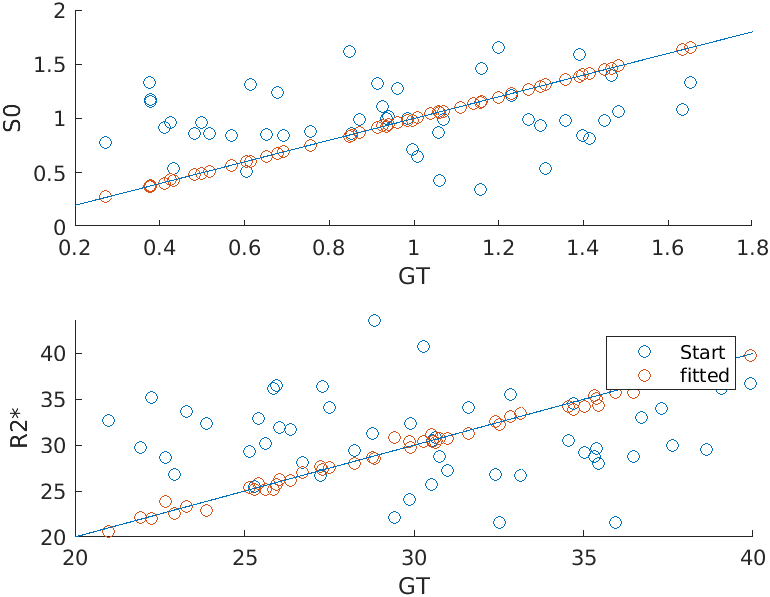
Scatterplots of the ground truth, starting points and estimation values
The full example script can be found in here.