askAdam basic tutorial for N-D data
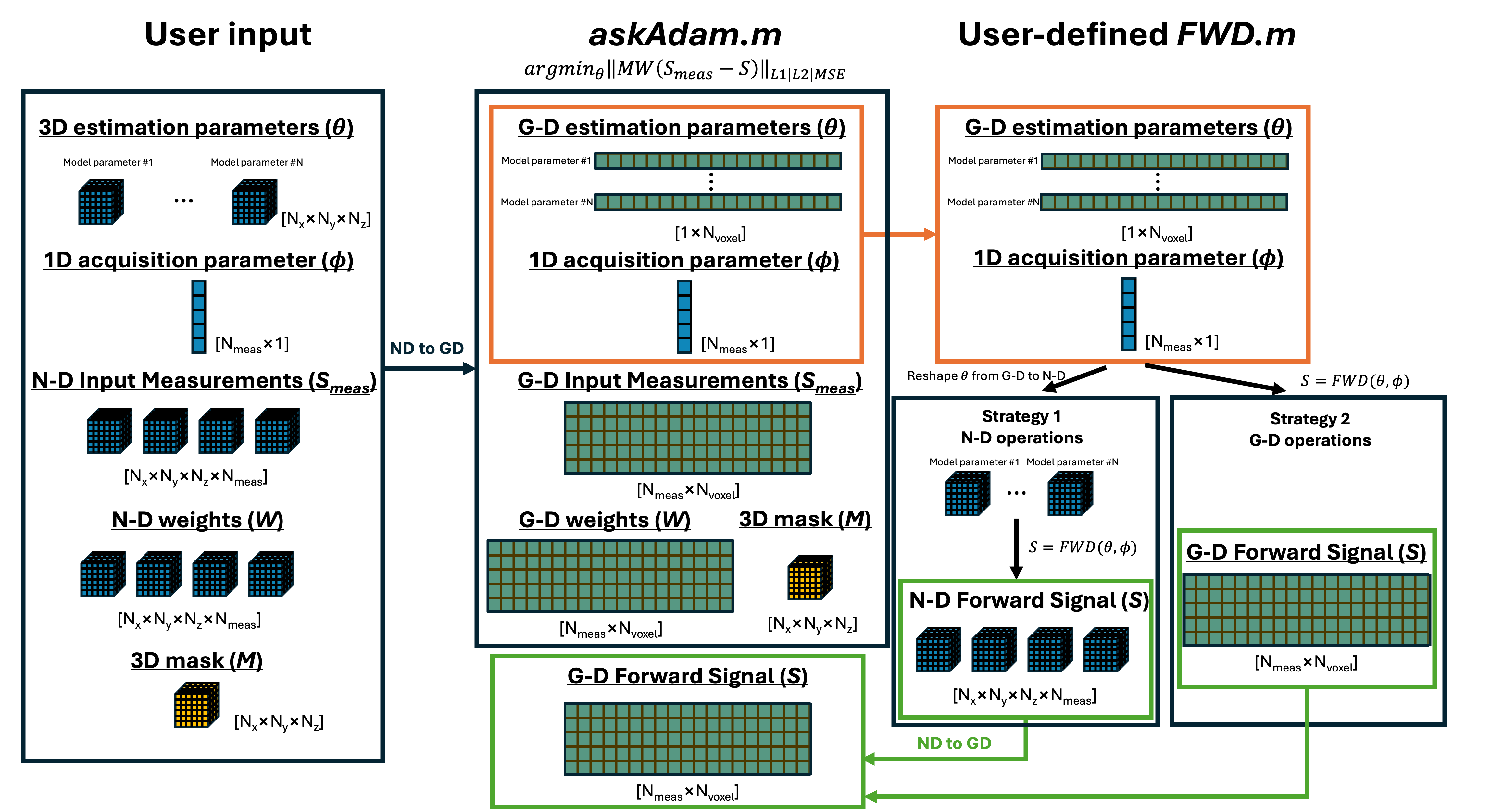
This tutorial demonstrates an example of how to use the askAdam solver in this package for model parameter estimation on N-D data (N>2). Here is the overview on how data size updates during the operation. Here we focus on the FWD.m column on the figure.
Let’s say we have a simple monoexponential decay model:
In this model, we have two parameters to be estimated: \(S0\) and \(R_{2}^{*}\).
Strategy 1
This strategy provides a more straightforward operation in terms of designing the signal model by making all operations N-D based. The drawback is that more GPU memory and computational power are needed.
The first thing is to create a function to generate the forward signal. To accomodate the first 3 dimensions for spatial information, we will put the time \(t\) in the 4th dimension.
Here is an example:
function S = Example_monoexponential_FWD_askadam_3D_Strategy1( pars, t)

% In this example we put the time in the 4th dimension
t = reshape(t(:),1,1,1,numel(t));

% S0 and R2tar are N-D array (1<=N<=3)
S0      = pars.S0;
R2star  = pars.R2star;

% compute S, as [Nx*Ny*Nz*Nt] matrix
S = S0 .* exp(-t.*R2star);

end
In contrast to the basic tutorial, we have some extra operations here
end
This block of code is to handle the input from askadam.m. As discussed in designing a new model, the estimation parameters from askAdam are already masked and reshaped into [1*Nvoxel] arrays. This block essentially has two operations: (1) checks if the estimation parameters are masked, (2) if so then reshape the estimation parameters to their original N-D size using the 3-D mask. GACELLE provides a utility function reshape_GD2ND to simplify the reshaping operation of an array from G-D size to N-D size.
Note that the final output S of this forward model function is always 4D ([Nx*Ny*Nz*Nt]). When S is not 2D, askadam.m will automatically apply the input mask internally.
We can then simulate the 4D measurements using this function
%% generate some signal based on monoexponential decay
% reproducibility
seed = 5438973; rng(seed); gpurng(seed);

% set up estimation parameters; must be the same as in FWD function
modelParams = {'S0','R2star'};

% define number of voxels and SNR
Nx      = 21;
Ny      = 21;
Nz      = 21;
SNR     = 100;
% let's create a spherical mask
mask        = strel('sphere',10);mask = mask.Neighborhood;
t           = linspace(0,40e-3,15);
% GT
S0          = 1 + randn(Nx,Ny,Nz)*0.3;
R2star      = 30 + 5*randn(Nx,Ny,Nz);
% forward signal generation
pars.(modelParams{1}) = S0;
pars.(modelParams{2}) = R2star;
% S now is a 4D matrix
S                     = Example_monoexponential_FWD_askadam_3D_Strategy1(pars,t);

% realistic signal with certain SNR
noise   = mean(S0(:)) / SNR;        % estimate noise level
y       = S + noise*randn(size(S)); % add Gaussian noise
Now y is our ‘realistic’ noisy data for the estimation.
This time we also have a spherical non-zero mask to demonstrate the usage of a mask.
mask = strel('sphere',10);mask = mask.Neighborhood;
To estimate \(S0\) and \(R_{2}^{*}\) from y,
Set up the starting point (pars0) for the estimation. pars0 has the same input format as pars of the forward function. In this example, we just use random values
pars0.(modelParams{1}) = 1 + randn(Nx,Ny,Nz)*0.5;  % S0
pars0.(modelParams{2}) = 20 + 10*randn(Nx,Ny,Nz);   % R2*
Set up the model parameters and fitting boundary
% set up fitting algorithm
fitting                     = [];
% define model parameter name and fitting boundary
fitting.modelParams         = {'S0','R2star'}; % modelParams;
fitting.lb                  = [0, 0];   % lower bound
fitting.ub                  = [2, 50];  % upper bound
Set up optimisation setting
% Estimation algorithm setting
fitting.iteration           = 4000;
fitting.initialLearnRate    = 0.001;
fitting.lossFunction        = 'l1';
fitting.tol                 = 1e-4;
fitting.convergenceValue    = 1e-8;
fitting.convergenceWindow   = 20;
fitting.isDisplay           = false;
Define the forward function
% define your forward model
Define fitting weights (optional)
% equal weights
Start the optimisation
askadam_obj = askadam;
Plot the estimation results
%% plot the estimation results
figure;
nexttile;scatter(S0(mask>0),pars0.(modelParams{1})(mask>0));hold on; scatter(S0(mask>0),out.final.S0(mask>0));refline(1);
xlabel('GT'); ylabel('S0')
nexttile;scatter(R2star(mask>0),pars0.(modelParams{2})(mask>0));hold on; scatter(R2star(mask>0),out.final.R2star(mask>0));refline(1)
xlabel('GT'); ylabel('R2*')
legend('Start','fitted')
figure; tiledlayout(2,3)
nexttile;imshow(S0(:,:,11).*mask(:,:,11),[0 2]);title('S0 GT')
nexttile;imshow(pars0.(modelParams{1})(:,:,11).*mask(:,:,11),[0 2]);title('S0 Start')
nexttile;imshow(out.final.S0(:,:,11),[0 2]);title('S0 Fitted')
nexttile;imshow(R2star(:,:,11).*mask(:,:,11),[10 60]);title('R2* GT')
nexttile;imshow(pars0.(modelParams{2})(:,:,11).*mask(:,:,11),[10 60]);title('R2* Start')

Center slice of the ground truth, starting points and estimation values

Scatterplots of the ground truth, starting points and estimation values
The full example script can be found in here.
Strategy 2
This strategy provides the most memory and computationally efficient way for the optimisation, but the operation is a bit less intuitive.
The first thing is to create a function to generate the forward signal. To accomodate the first 3 dimensions for spatial information, we will put the time \(t\) in the 4th dimension.
Here is an example:
 1function S = Example_monoexponential_FWD_askadam_3D_Strategy2( pars, t, mask)
 2
 3% In this example we put the time in the 4th dimension
 4t = reshape(t(:),1,1,1,numel(t));
 5
 6% S0 and R2tar are N-D array (1<=N<=3)
 7S0      = pars.S0;
 8R2star  = pars.R2star;
 9
10% compute S, as [Nx*Ny*Nz*Nt] matrix
11S = S0 .* exp(-t.*R2star);
12
13%%%%%%%%%%%%%%%%%%%%%%%%%%%%%%%%%%%%%%%%%%%%%%%%%%%%%%%%
14% to maximise the GPU memory efficiency, pars.S0 and pars.R2star are masked inside askAdam.m by default, therefore they have size of [1*Nvoxel]
15% that means the size of S will be [1*Nvoxel*1*Nt] during the askAdam optimisation loops
16% since S only contains the masked voxel, we need to convert S into a 2D array to avoid additional masking step in askAdam.m
17% the utility function 'reshape_ND2GD' can convert any N-D array (N>=4) into 2D array ([Nmeas*Nvoxel]) compatible for askAdam.m
18% compare to Strategy 1 this is a more memory efficient way since fewer total voxels are involved but less intuitive
19if any(size(S0,1:3) ~= size(mask,1:3))  % if the size doesn't match then the input is masked
20    S = utils.reshape_ND2GD(S,[]);
21end
22%%%%%%%%%%%%%%%%%%%%%%%%%%%%%%%%%%%%%%%%%%%%%%%%%%%%%%%%
23
24end
In contrast to the basic tutorial, we have some extra operations here
if any(size(S0,1:3) ~= size(mask,1:3))  % if the size doesn't match then the input is masked
    S = utils.reshape_ND2GD(S,[]);
end
This block of code is to handle the input from askadam.m. As discussed in designing a new model, the estimation parameters from askAdam are already masked and reshaped into [1*Nvoxel] arrays. This block essentially has two operations: (1) checks if the estimation parameters are masked, (2) if so then reshape the output S to the G-D format. GACELLE provides a utility function reshape_ND2GD to simplify the reshaping operation of an array from the N-D size to G-D size.
Note that the idea of the function design here is a bit different from Strategy 1: In Strategy 1, we make sure the output for the forward function is (4)N-D and let askadam.m deals with the masking internally. In Strategy 2, we accepted the masked estimation parameters in G-D format from askadam.m and make sure the output S is also in G-D format in the optimisation process.
Note that the size of S can be G-D or N-D, depending on whether the estimation parameters stired in the input variable pars are G-D or N-D. The output variable S at Line 11 is still in 4D format regardless the size of \(S0\) and \(R_{2}^*\).
We can then simulate the 4D measurements using this function by using 3D \(S0\) and \(R_{2}^*\) input.
%% generate some signal based on monoexponential decay
% reproducibility
seed = 5438973; rng(seed); gpurng(seed);

% set up estimation parameters; must be the same as in FWD function
modelParams = {'S0','R2star'};

% define number of voxels and SNR
Nx      = 21;
Ny      = 21;
Nz      = 21;
SNR     = 100;
% let's create a spherical mask
mask        = strel('sphere',10);mask = mask.Neighborhood;
t           = linspace(0,40e-3,15);
% GT
S0          = 1 + randn(Nx,Ny,Nz)*0.3;
R2star      = 30 + 5*randn(Nx,Ny,Nz);
% forward signal generation
pars.(modelParams{1}) = S0;
pars.(modelParams{2}) = R2star;
% S now is a 4D matrix
S                     = Example_monoexponential_FWD_askadam_3D_Strategy2(pars,t,mask);

% realistic signal with certain SNR
noise   = mean(S0(:)) / SNR;        % estimate noise level
y       = S + noise*randn(size(S)); % add Gaussian noise
Now y is our ‘realistic’ 4D noisy data for the estimation.
This time we also have a spherical non-zero mask to demonstrate the usage of a mask.
mask = strel('sphere',10);mask = mask.Neighborhood;
To estimate \(S0\) and \(R_{2}^{*}\) from y,
Set up the starting point (pars0) for the estimation. pars0 has the same input structure organisation as pars of the forward function. It can be N-D array as the same way we generated y. In this example, we just use random values
pars0.(modelParams{1}) = 1 + randn(Nx,Ny,Nz)*0.5;  % S0
pars0.(modelParams{2}) = 20 + 10*randn(Nx,Ny,Nz);   % R2*
Set up the model parameters and fitting boundary
% set up fitting algorithm
fitting                     = [];
% define model parameter name and fitting boundary
fitting.modelParams         = {'S0','R2star'}; % modelParams;
fitting.lb                  = [0, 0];   % lower bound
fitting.ub                  = [2, 50];  % upper bound
Set up optimisation setting
% Estimation algorithm setting
fitting.iteration           = 4000;
fitting.initialLearnRate    = 0.001;
fitting.lossFunction        = 'l1';
fitting.tol                 = 1e-4;
fitting.convergenceValue    = 1e-8;
fitting.convergenceWindow   = 20;
fitting.isDisplay           = false;
Define the forward function
% define your forward model
Define fitting weights (optional)
% equal weights
Start the optimisation
askadam_obj = askadam;
Plot the estimation results
%% plot the estimation results
figure;
nexttile;scatter(S0(mask>0),pars0.(modelParams{1})(mask>0));hold on; scatter(S0(mask>0),out.final.S0(mask>0));refline(1);
xlabel('GT'); ylabel('S0')
nexttile;scatter(R2star(mask>0),pars0.(modelParams{2})(mask>0));hold on; scatter(R2star(mask>0),out.final.R2star(mask>0));refline(1)
xlabel('GT'); ylabel('R2*')
legend('Start','fitted')
figure; tiledlayout(2,3)
nexttile;imshow(S0(:,:,11).*mask(:,:,11),[0 2]);title('S0 GT')
nexttile;imshow(pars0.(modelParams{1})(:,:,11).*mask(:,:,11),[0 2]);title('S0 Start')
nexttile;imshow(out.final.S0(:,:,11),[0 2]);title('S0 Fitted')
nexttile;imshow(R2star(:,:,11).*mask(:,:,11),[10 60]);title('R2* GT')
nexttile;imshow(pars0.(modelParams{2})(:,:,11).*mask(:,:,11),[10 60]);title('R2* Start')
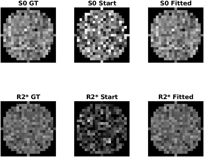
Center slice of the ground truth, starting points and estimation values
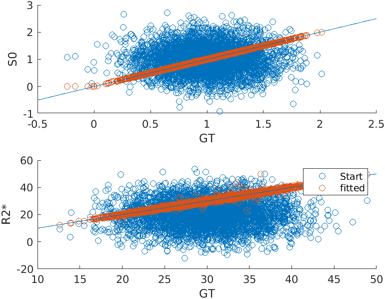
Scatterplots of the ground truth, starting points and estimation values
These results are exactly the same as Strategy 1 because we used the same seed and mask.
The full example script can be found in here.