askAdam basic tutorial

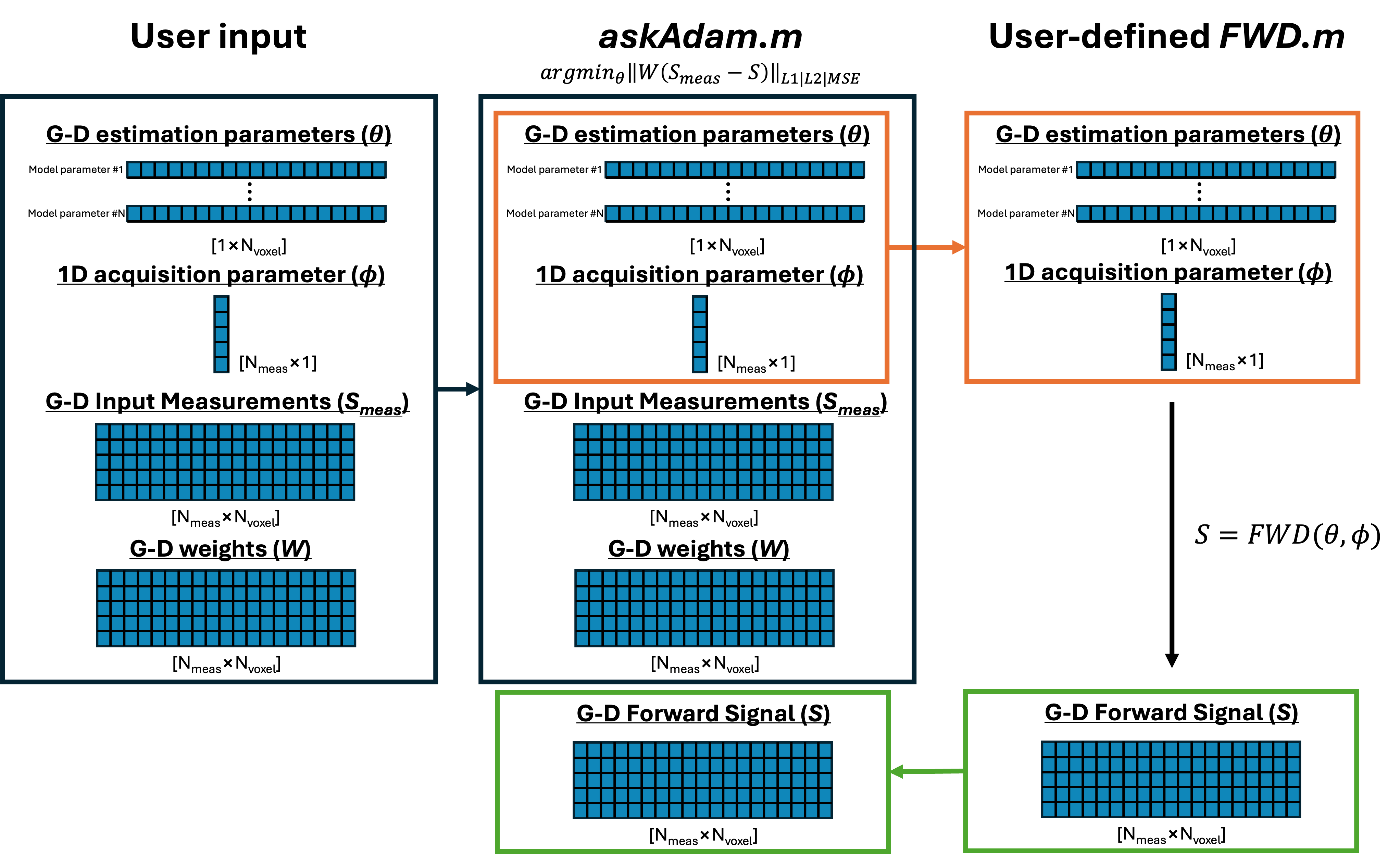
This tutorial demonstrates an example of how to use the askAdam solver in this package for model parameter estimation, based on the G-D input option shown in here:

Let’s say we have a simple monoexponential decay model:

\[S = S0 \times e^{-R_{2}^{*}t}\]

In this model, we have two parameters to be estimated: \(S0\) and \(R_{2}^{*}\).

The first thing is to create a function to generate the forward signal. Here is an example:

function S = Example_monoexponential_FWD_GD( pars, t)
    
% columnised t
t = t(:);

% S0 and R2star here are [1xNvoxel] arrays
S0      = pars.S0;
R2star  = pars.R2star;

% compute S, as [NtxNvoxel] matrix
S = S0 .* exp(-t.*R2star);

end

Note that this function takes in two input variables: pars and t, where pars is a structure variable stored 2 fields: S0 and R2star, with a size of [1*Nvoxel], and t are the echo times of the measurments. The output variable S is a time decay signal with a size of [Nt*Nvoxel].

We can simulate the measurements using this function

%% generate some signal based on monoexponential decay
% reproducibility
seed = 5438973; rng(seed); gpurng(seed);

% set up estimation parameter name; must be the same as the fields of 'pars' in the forward function
modelParams = {'S0','R2star'};

% define number of voxels and SNR
Nsample = 100;
SNR     = 100;

mask        = ones(1,Nsample)>0;
t           = linspace(0,40e-3,15); 
% GT
S0          = 1 + randn(1,Nsample)*0.3;
R2star      = 30 + 5*randn(1,Nsample);
% forward signal generation
pars.(modelParams{1}) = S0; 
pars.(modelParams{2}) = R2star;
S = Example_monoexponential_FWD_GD(pars,t);

% realistic signal with certain SNR
noise   = mean(S0) / SNR;           % estimate noise level
y       = S + noise*randn(size(S)); % add Gaussian noise

Now y is our ‘realistic’ noisy data for the estimation.

Note

The dimenion and arrangement of y must be the same as the output S of the forward function.

To estimate \(S0\) and \(R_{2}^{*}\) from y,

1. Set up the starting point (pars0) for the estimation. pars0 has the same input format as pars of the forward function. In this example, we just use random values

pars0.(modelParams{1}) = 1 + randn(1,Nsample)*0.5;  % S0
pars0.(modelParams{2}) = 20 + 10*randn(1,Nsample);   % R2*

2. Set up the model parameters and fitting boundary.

% set up fitting algorithm
fitting                     = [];
% define model parameter name and fitting boundary
fitting.modelParams         = {'S0','R2star'}; % modelParams;
fitting.lb                  = [0, 0];   % lower bound 
fitting.ub                  = [2, 50];  % upper bound

3. Set up optimisation setting

% Estimation algorithm setting
fitting.iteration           = 4000;
fitting.initialLearnRate    = 0.001;
fitting.lossFunction        = 'l1';
fitting.tol                 = 1e-4;
fitting.convergenceValue    = 1e-8;
fitting.convergenceWindow   = 20;
fitting.isDisplay           = false;

4. Define the forward function

% define your forward model
modelFWD = @Example_monoexponential_FWD_GD;

5. Define fitting weights (optional)

% equal weights
weights = [];

6. Start the optimisation

askadam_obj = askadam;
out         = askadam_obj.optimisation(y,mask,weights,pars0,fitting,modelFWD,t);

7. Plot the estimation results

%% plot the estimation results
figure;
nexttile;scatter(S0,pars0.(modelParams{1}));hold on; scatter(S0,out.final.S0);refline(1);
xlabel('GT'); ylabel('S0')
nexttile;scatter(R2star,pars0.(modelParams{2}));hold on; scatter(R2star,out.final.R2star);refline(1)
xlabel('GT'); ylabel('R2*')
legend('Start','fitted')

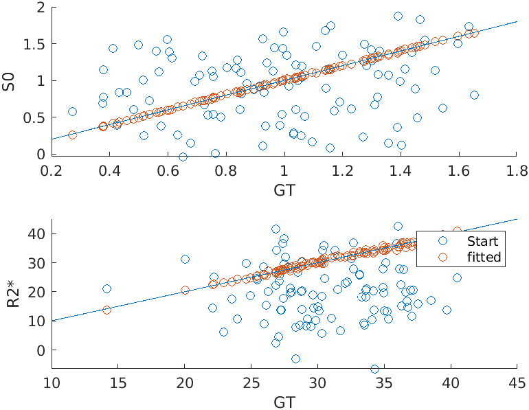
Scatterplots of the ground truth, starting points and estimation values

The full example script can be found in here.